Cohen (1994) – The Earth Is Round (p < .05)

Main focus of the article: In this article the author presents his arguments on what is wrong with Null Hypothesis Significance Testing (NHST) and suggests ways in which researchers can improve their research and reporting thereof.

---

My comments on the article:
Cohen argues that “NHST has not only failed to support the advance of psychology as a science but also has seriously impeded it” (p. 997). It is clear that he is not a fan of NHST, although he indicates that this was not always so. Cohen asks the question “What’s wrong with NHST?” and proceeds to answer it with “… it does not tell us what we want to know …” (p. 997). It is true that NHST does not give us the    or even    which is typically what we would like to know. Instead, NHST gives us    from which we make an inference about what is possibly happening in the underlying population.

The Permanent Illusion

Cohen cites Falk & Greenbaum (1995) (in press at the time) along with Gigerenzer (1993) in referring to the “illusion” created in the logic of NHST. Cohen, like Falk & Greenbaum and many others, imply that the logic of NHST is somehow a formal mathematical proof. Cohen then uses an example of the logic of a modus tollens proof to demonstrate how the imprudent insertion of the word “probably” can lead to erroneous results. By the same argument, Cohen then suggests that this is the flaw in the reasoning of NHST. However, the logic of NHST is not a modus tollens proof and this is the problem with the use of this argument against the use of NHST. To be clear, a formal mathematical proof results in a definitive conclusion (e.g.    is irrational) whereas the conclusions of NHST still contain uncertainty.

Why P(D|H₀) ≠ P(H₀|D)

Cohen then goes on to discuss the problems associated with the fact that (most of the time)   . Cohen states that “what is always the real issue, is the probability that    is true, given the data, [    ], the inverse probability” (p. 998). Whilst it is true that in many cases one would like to obtain the inverse probability, it is also true that in many cases, particularly in debunking claims, one is more interested in   . It stands to reason that if you are interested in determining the    then NHST is the wrong technique to use. This does not mean that NHST is faulty, but that it is not designed to provide that probability.

Cohen then discusses a screening test for schizophrenia and how this “demonstrates how wrong one can be by considering the p-value from a typical significance test as bearing on the truth of the null hypothesis for a set of data” (p. 999). This comparison that Cohen and many others have used in arguing against NHST is an “apples and oranges” comparison and is grossly misleading. The temptation to make this comparison perhaps comes from the fact that there are four possible outcomes in a hypothesis test (correctly/incorrectly rejecting/failing to reject   ) and four parameters of a screening test (true/false positive/negative). Whilst there are similarities, it should be clear that the Type I error rate (  ) of a hypothesis test is not directly comparable with the false positive rate of a screening test.

Firstly, in NHST the true value of the population parameter is unknown. It is assumed that    is true, which is the hypothesis of the status quo, giving a value for the population parameter needed for computing the resulting p-value. Secondly, the a priori significance level (  ), also called the Type I error rate, is a subjective choice of the researcher. Thirdly, the Type II error rate (  ) is, ceteris paribus, a function of the difference between the distribution under the Null Hypothesis and the true distribution, the sample size (  ) and the selected Type I error rate (  ). The researcher can affect the value of the Type II error rate by simply adjusting the sample size. Compare this to a screening test where the false positive (similar to a Type I error) rate is a property of the test and cannot be selected by the researcher. Equally, the false negative (similar to a Type II error) rate is also a property of the test and is unaffected by increasing the sample size. As such comparing NHST to a screening test in the manner of Cohen and others will lead a reader to an erroneous conclusion, whether deliberately or unintentionally.

Fortunately Cohen does spell out to the reader that NHST does have a place in falsifying theories and clarifies that his criticism is aimed at the use of it to “confirm” theories through “rejecting null hypotheses” (p. 999). Here I definitely agree with Cohen in that NHST does not confirm the Alternate Hypothesis (often called the Research Hypothesis in psychology) when the null is rejected. This misconception, as Cohen and others state, unfortunately appears in many textbooks and research articles. The reason behind this misconception is perhaps mostly due to an innate desire to conclude that if the null hypothesis is not supported it must therefore be false and if the null is false, the alternate must therefore be true, what Cohen calls the “Bayesian Id” (p. 999). No doubt I have been guilty of falling into this trap in the past and it takes a good deal of vigilance not to fall into it again when working with uncertainty. Uncertainty is not something we human beings seem comfortable with, nor something we appear to be well equipped to reason with as is evidenced by the multitude of times such misconceptions are published even in reputable journals.

Cohen’s main argument against NHST appears to be in how it is misused, rather than with it’s design. NHST is not designed to, nor is it meant to, be used in confirming a theory. Hence, calling for the abandonment or prohibition on the use of NHST because of misuse is akin to calling for the abandonment or prohibition on the use of the Internet because of illegal downloading. What is needed, in my opinion, is better education of those using NHST to understand what it can and cannot do. Equally, those who need to learn about NHST should also be instructed in alternatives such as Bayesian Inference.

Naturally, to ensure that this instruction is done thoroughly and correctly, students should be required to undertake studies in statistics, taught by professional statisticians, throughout their degree programs. Unfortunately, most students who need to use statistics in their disciplines are only required to undertake one semester of such studies, typically in their first year, and rarely does this cover more than the very basics of inferential techniques. The tragedy of this situation is that these students are not properly exposed to alternative analysis techniques available to suit situations where NHST is not appropriate; nor are these students given opportunity to acquire even adequate skills in reasoning with uncertainty, statistical and critical thinking – the core skills of robust and rigourous science. It is little wonder then that many of these students end up believing such misconceptions as that the “p-value is the probability that    is true”.

The Nil Hypothesis

Cohen states that “as almost universally used, the null in    is taken to mean nil, zero” (p. 1000). I would disagree that this is “universal” and certainly not what I teach. The null hypothesis is the hypothesis of the status quo, no change or no difference to the effect. In real world research, such as drug trials, this does often mean zero effect (i.e. no better than placebo), but it is not required to mean zero effect. There is nothing in the mathematics of computing a two-sample t-test, for example, that requires   . Cohen states that “most of the criticism of NHST in the literature has been for this special case where its use may be valid only for true experiments using [randomisation]” but that “even in these cases, confidence intervals provide more information” (p. 1000). Confidence Intervals, themselves often misinterpreted and misreported, do provide a likelihood interval for the parameter of interest, but are based on the same Null Hypothesis and utilise the same mathematics p-values and are, in fact, part of NHST. As such, they do not provide different information from NHST.

Cohen introduces what he calls the “Nil Hypothesis” to mean the hypothesis of zero effect size. Cohen, as indicated by the previous quote, believes that this hypothesis can only be used in situations, i.e. those “special cases”, where one has reasonable grounds to expect a zero effect size, but that it should not be used for most research scenarios. Here I agree with Cohen in that the Null Hypothesis in every hypothesis test should reflect the expected situation under the assumption that nothing has changed, but then this is the theory of NHST. Unfortunately, most textbooks fail to place sufficient emphasis on this fact, indeed some actually misrepresent the theory of certain tests completely. Take, for example, the paired t-test as presented in the Aron, Aron and Coups text “Statistics for the Behavioral and Social Sciences“. The authors state that “Saying there is on average no difference is the same as saying that the mean of the population of difference scores is 0” and then later in the same paragraph, “In other words, with a t-test for dependent means, what we call Population 2 will ordinarily have a mean of 0″ (p. 247). The formula then presented to the student in the summary of steps for this test is

     i.e.   

Leaving aside the confusion created by the APA convention to use capital letters for sample statistics, this formula does not allow for the testing of anything other than zero difference. As such, despite Aron, Aron and Coups’ statement that it will “ordinarily have a mean of 0″, the presented formula implies that it will always have a mean of 0. The poor students using this text, and others like it, are then left with the impression that one can only test for a mean of 0. Little wonder then that Cohen laments the use of the “Nil Hypothesis” in situations where this is clearly ridiculous.

Cohen goes on to state that “the nil hypothesis is always false” (p. 1000), however, I would argue that the reasoning behind this statement is incorrect. If, as Cohen states, “it is false, even to a tiny degree, it must be the case that a large enough sample size will produce a significant result and lead to its rejection. So if the null hypothesis is always false, what’s the big deal about rejecting it?” (p. 1000). The problem with this line of argument is that it implies that any population parameter value chosen for the Null Hypothesis is false, even the unknown true value of the population parameter. If that is the case, why bother testing, or evening measuring values at all? They are all wrong!

It is true that for any continuous function    the integral for any point    is    and thus if population    has density function    (i.e. non-discrete distribution) then   . Therefore one could argue that any point estimate of a population parameter (or effect size) is false by the same logic, however, we know that the population parameter must take some value. Equally, we also know that for    to be a valid probability density function, the total area under the curve must equal to 1 (i.e.   ). For that to be true,    must be non-zero for at least one value of    in the domain.

What we need to bear in mind here is that NHST is about trying to determine if there is sufficient evidence to reject the assumption that nothing has changed. If we already know that the effect size is non-zero, then why would you set your Null Hypothesis to test if it is zero? Equally if past research suggests the value of the effect size why would you set your Null Hypothesis to test any other value? What is typically overlooked in these arguments about the Null Hypothesis always being false is difference between the theoretical “it is always false” and practical “it must take some value” and that there will be some uncertainty in our measurements of such values.

We might state that the parameter equals 5 (in theory), but what we mean is that it equals 5 within the tolerances of our measurement precision (i.e. in practice). Cohen highlights the issue of precision indirectly when he quotes Tukey (1991), “It is foolish to ask ‘Are the effects of A and B different?’ They are always different – for some decimal place” (p. 1000). In a similar way to the argument that two values will differ in some decimal place, so to will any measurement we make be incorrect at some decimal place. What is important to recognise is that our measurements will be precise to some level of tolerance and so check them only to that level of precision or lower. Equally, researchers should be aware that the precision of their sample statistic is proportional to the reciprocal of the square root of the sample size (i.e.   ). Hence this is yet another reason why it is important to take large samples.

Cohen goes on to cite Thompson (1992), “Statistical significance testing can involve a tautological logic in which tired researchers, having collected data on hundreds of subjects, then conduct a statistical test to evaluate whether there were a lot of subjects, which the researchers already know, because they collected the data and know they are tired. This tautology has created considerable damage as regards the cumulation of knowledge. (p. 436)” (p. 1000). Here I would argue that Cohen through Thompson is demonstrating that there is a problem with how statistical tests are being used, not really suggesting a problem with the tests themselves. Researchers should not collect the data and then perform a statistical test, statistical testing begins before data is collected, not afterwards!

Before a researcher goes off to collect any data to make inferences, they must have a research question and therefore have determined: (a) their statistical hypotheses, the statistical technique(s) used to test them and the conditions for inference; (b) their research design (in order to best satisfy the conditions of inference); and, (c) the sample size required for their chosen significance level, desired power and estimated expected effect size. If the research involves animals or human beings, the ethics committee should have already asked the researcher to provide this information before approving the research and allowing data to be collected. If the appropriate background work is done, then there is nothing tautological in performing NHST. If, however, the researcher simply collects data and then attempts to perform statistical tests on this data, I would argue that, aside from being poor scientific practice, they should not be trying to generalise beyond the sample data in any case. In such circumstances, the best thing for the researcher to do, in my opinion, is to write a descriptive piece about their collected data and indicate what the data suggests as future lines of enquiry.

Cohen then discusses an unpublished study by Meehl and Lykken which looked at a data set of “15 items for a sample of 57,000 Minnesota high school students” (p. 1000) as evidence of how bad the Nil Hypothesis is for research. In this study the researchers apparently have performed 105 pairwise cross-tabulations and all were “statistically significant, and 96% of them [with] p < [0].000001″ (p. 1000). Presumably the authors were testing at an overall 5% level of significance (  ) as is typically used in non-life threatening research like this. Equally, one would presume that Meehl and Lykken have made the necessary Bonferroni corrections to their alpha level for each of the planned pairwise comparisons so that each is individually checked at no more than   . Even so, the biggest problem with this study, as it is presented, is that Meehl and Lykken are unlikely to have ensured that each of the students were independent of one another (i.e. unrelated) before including them in the study since that is a condition of inference for Chi-squared cross-tabulations. After all, the Chi-squared cross-tabulation test that they have used, is trying to assess if there is an association between the item pairs. If two students are siblings then they will have the same parents and therefore the same responses on at least 5 of the listed items and related responses on at least 1 other item. Also, given that all of the students are drawn from the same state of Minnesota, there is likely to be commonalities in opinions due to shared community experiences, morals and values. In addition, there is likely to be some homogeneity with regards to an item like “high school organisations”, since students at the same school will have access to only those organisations offered at that school. Hence if the data contains many related samples, I would not find it surprising that the results are statistically significant in all 105 pairwise comparisons, even at the    level.

Cohen states that, “Meta-analysis, with its emphasis on effect sizes, is a bright spot in the contemporary scene” (p. 1000). Meta-analysis, it is true, does focus on effect sizes, however, it is used for a different purpose than NHST in that it looks at the results of multiple (hopefully independent) research studies. In that regard it is further down the chain in the “Scientific Method” than a single research study and therefore not directly comparable to NHST.

Leaving that aside, Cohen then presents the fallacious reasoning that since “the nil hypothesis is always false, the rate of Type I errors is 0%, not 5%” (p. 1000). Here Cohen has basically argued that since the “nil” hypothesis is always false, that it then follows that   . From basic probability theory we know that the conditional probability is given by    which, in the case of a Type I error would be   . If, as according to Cohen and others,    then the Type I error rate would involve a division by zero and hence would be undefined and not equal to zero as claimed.

Again, it is important to understand what a Type I (  ) and Type II (  ) error actually are. A Type I error is committed when one rejects the Null Hypothesis when it is in fact true. In other words, when it is concluded that things have changed when in fact they have not. A Type II error is committed when we fail to reject the Null Hypothesis when it is in fact false. In other words, when it is concluded that things have not changed when in fact they have. In practice we don’t know if the Null Hypothesis is really true or false, so we don’t ever know if we have made either of these two kinds of errors. As such, we try to minimise the probability of making either error, however, more emphasis is placed upon minimising the Type I error rate. This emphasis is due to the fact that a Type I error is akin to claiming that you have found evidence of an effect when the effect does not in fact exist.

Cohen argues that “there is the irony that the “sophisticates” who use procedures to adjust their alpha error for multiple tests (using Bonferroni, Newman-Keuls, etc.) are adjusting for nonexistent alpha error, thus reduce their power, and, if lucky enough to get a significant result, only end up grossly overestimating the population effect size!” (p. 1000). Here I would again disagree with Cohen, since there is nothing nonexistent about the Type I error unless you subscribe to the fallacy the Null Hypothesis is always false. Despite Cohen’s implication too, there is nothing sophisticated about adjusting for multiple comparisons, rather it is a necessary step to ensure that one does not inflate the probability of making a Type I error. It may be true that the subsequent estimates of population effect size are overestimates or underestimates, but since the true population effect size is almost always unknown, what we need is the minimum variance unbiased estimator (MVUE) of the effect size. In a similar way to selecting the correct statistical test, one must take care in selecting the correct measure of effect size.

Cohen states that “Because NHST p-values have become the coin of the realm in much of psychology, they have served to inhibit its development as a science” (p. 1001). It could hardly be the fault of p-values that any discipline is inhibited in its scientific development, but rather the poor understanding and misuse of such values. Cohen goes on to state that “psychologists know that statistically significant does not mean plain-English significant” (i.e. important), but that the literature suggest otherwise (p. 1001). Like Cohen, I too would argue that the research literature (and indeed my own experiences in consulting with researchers) demonstrates quite the opposite and that those who understand significant does not mean important are the exception, not the norm.

Cohen then argues that “Even a correct interpretation of p-values does not achieve very much, and has not for a long time” (p. 1001). This statement, and the supporting arguments that follow, suggest that the main concern Cohen has about p-values and NHST is that they don’t do much when misused. A p-value is not designed to tell you if the difference between A and B is important or how large it is, rather it is designed to tell you if there is enough evidence to reject the assumption that nothing has changed. Additional information, such as the estimated effect size or underlying theory, is required to tell you if this result is important, theoretically or practically. Like in a murder investigation, the suspect simply not having alibi for the time of the crime may or may not be important, additional information is required before charges are laid.

Reading this portion of the article it becomes more apparent that Cohen’s main argument with NHST appears to be only about the misuse of such techniques. The citation of Tukey (1969) demonstrates this clearly as Tukey discusses how one needs to make measurements of size not simply direction. NHST is designed to indicate if there is sufficient evidence to reject the assumption that nothing has changed, not to make measurements of size. Once you have rejected the assumption that nothing has changed (i.e. the Null Hypothesis), one can then use the sample data to estimate the effect size. This measurement, combined with other replications of the same experiment that yield their own estimated effect sizes, can then be used to develop new theories.

Curiously, when discussing correlation coefficients and his own effect size measures, Cohen advises the reader that “like correlations, also dependent on population variability of the dependent variable and are properly used only when that fact is kept in mind” (p. 1001). In my experience, I have observed that many researchers report correlation coefficients for their data, clearly forgetting that measures like Pearson’s r measure the strength and direction of the linear association between two quantitative variables. It is not uncommon, particularly in disciplines involving animal or human subjects, to see a Pearson’s r statistic for the association between gender and some other variable or for some non-linear relationship. Equally worrying about Cohen’s discussion on correlation coefficients is the statement that the “major problem with correlations applied to research data is that they can not provide useful information on the causal strength because they change with the degree of variability of the variables they relate. Causality operates on single instances, not on populations whose members vary” (p. 1001). Correlation does not imply causation and nor is the correlation coefficient meant to measure the strength of causation. Similarly, determining a causal link requires a true-experimental research design with strong controls whereas correlations can be determined under much looser conditions, even using historical data.

Cohen’s last statement in this section worryingly demonstrates the erroneous thinking often seen with correlation and regression, “Recall my example of the highly significant correlation between height and intelligence in 14,000 school children that translated into a regression coefficient that meant that to raise a child’s IQ from 100 to 130 would require giving enough growth hormone to raise his or her height by 14 feet (Cohen, 1990)” (p. 1001). Aside from the error of equating correlation with causation (i.e. that height causes IQ), it is dangerous to extrapolate beyond the range of the sample data and hence why the model would give the ridiculous value of needing an additional 14 feet. I would wonder at what height the model began giving negative values for IQ or how Cohen would interpret the intercept term in such a model (i.e. when height is zero).

What to Do?

Cohen provides three suggestions for his readers, the first being not to look for some magic alternative to NHST. I think it would have been better if he had stated “Remember to use the right tool for the right job” rather than to suggest not looking for an alternative. His second suggestion to use Exploratory Data Analysis (EDA) techniques is also greatly concerning. As Cohen states, EDA is mostly based on graphical techniques aimed at gaining an intuitive interpretation of observations. Given the problems that most non-statisticians have in understanding simple techniques like correlation and regression, suggesting that researchers use their intuition is fraught with danger. To demonstrate, take the following scenario from my own teaching materials on Two-Way Analysis of Variance (ANOVA). In this scenario, students (mostly studying psychology) are looking to answer the research question ‘Is there an optimal combination of exercise program and behavioural modification technique on time between bad behaviours for disruptive children?’. Students are instructed in the techniques of Two-Way ANOVA and then as part of the reinforcement of the differences between intuition and evidence, are shown the following graph.

Intuitively, one would interpret this graph as suggesting that there is an interaction between the two independent variables (in the population) because the lines cross and if EDA were all that was used, then that would be what was reported. However, the statistical test for the interaction shows that this interaction is not statistically significant at the 5% level with 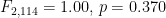  . Therein lies the danger of relying solely on intuition.

Cohen’s third suggestion is for researchers to “routinely report effect sizes in the form of confidence limits” (p. 1002). This suggestion I can certainly agree with, although with a word of caution. One of the biggest challenges in communicating statistical results is in ensuring that the reader understands what is being said. The term “Confidence” is often associated with certainty, whereas when we report a Confidence Interval, the confidence is in the method used to generate the interval, not in the values of that interval. Such lexical challenges to the reader’s understanding are widespread in statistical analysis and it is only through greater education, in my opinion, that such challenges will be met. In the meantime, the best thing researchers can do to improve their research is to consult with a professional statistician before they start collecting data or even designing their research project. This will help to avoid many of the problems brought about by using the wrong technique or misusing/misinterpretting a technique.

Full citation and link to document:
Cohen, J. (1994). The Earth Is Round (p < .05). American Psychologist, 49(12), 997-1003. doi:10.1037/0003-066X.49.12.997

 

CITE THIS AS:  
Ovens, Matthew. “Cohen (1994) The Earth Is Round (p < .05)” Retrieved from YourStatsGuru.

First published 2012 | Last updated: 19 June 2018